Calculation Example of Daily Indices

1VOL Index

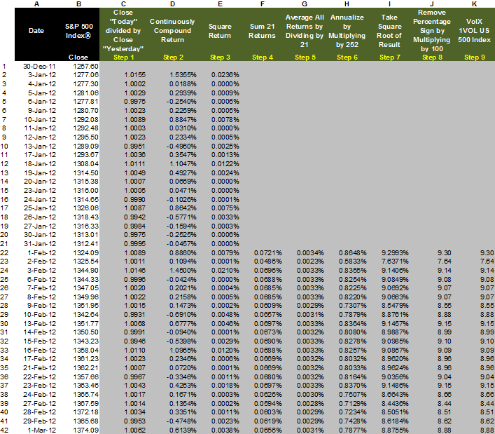
The following is a step-by-step description of the daily 1VOL index-calculation methodology. Note: The following refer to Exhibit 2. Also note that the spreadsheet contains data through 1 March 2012.

In column A are trading dates. Weekends and holidays are removed because the calculation ignores those days.
In column B are the closing prices of the underlying corresponding to the date in column A. In this particular case, we use the S&P 500 Index® as the underlying, but any underlying with a daily closing price is possible.
In column C is “today’s” closing price divided by “yesterday’s” closing price. Specifically, cell C2 has the formula “=B2/B1”. This cell is copied down the column such that cell C3 has the formula “=B3/B2”, etc. (Excel changes the reference cells automatically as the initial formula is copied down the spreadsheet.)
In column D is the continuously compounded return of each value in column C. The formula in cell D2 is “=LN(C2)”. Again, this formula is copied down the column and Excel changes the references automatically to the next cell such that cell D3 will now contain the formula “=LN(C3)”, etc.
In column E is the squared return. The formula in column E2 is “=D2^2”. Note: the “^” symbol means “to raise the variable to the power of.” So, D2^2 is equal to the square of D2 (or D2*D2). Again, this cell is copied down the column and Excel changes the relative references.
In column F is the sum of the previous 21 days’ returns. The formula in cell F22 is “=SUM(E2:E22)”. In Excel, the “SUM” function adds all items within the parentheses. And, in this case, “E2:E22” is the accepted notation to include everything in the cell starting with E2 and continuing in order through E22. Therefore, the “=SUM(E2:E22)” is equivalent to “=SUM(E2,E3,E4,E5,…,E22)”, and in mathematical notation, this is equivalent to E2+E3+E4+E5+…+E22. The formula gets copied down the page in a similar manner as described above. Excel automatically changes the formula reference each time such that cell F23 would have the formula “=SUM(E3:E23)”, etc.
In column G is the average of the 21 days’ returns. To get the average, divide each value in column F by 21. The formula in G22 is “=F22/21”. Again, this value is copied down the column.
In column H is the annualization factor. To annualize the value, just multiply each value in column G by 252 (the approximate number of trading days in a year). The formula in cell H22 is “=G22*252”. Note: The symbol “*” means to multiply. Again, copy the formula down the column.
In column I is the square root of each value in column H. The formula in cell I22 is “=SQRT(H22)”. “SQRT” is the built-in function in Excel that takes the square root of the number within the parentheses. Again, this cell is copied down the column.
In column J is the removal of the percentage sign by multiplying the result in column I by 100. The formula in cell J22 is “=I22*100”.
In column K is the “Daily 1VOL U.S. 500 Index.” The formula in K22 is “=J22”.

As you will notice, it takes 22 days of closing prices to calculate 21 days of returns. And, the first 21 returns are needed in order to calculate the very first 1VOL index value. Therefore, whatever URPs are used, a 1VOL index cannot produce its very first value until 21 days have passed. However, please note that this is a one-time issue. The S&P 500 index has been available in its current form since 1957 (the author believes that the index was actually started in January 1957). Therefore, the 1VOL index based on the underlying of S&P 500 index can be calculated back to February 1957 (approximately one month after the launch of the underlying) and would be continuous since then.

For clarification, the example in Exhibit 2 shows that the 1VOL index started in Feb 2012. This was done simply for explanatory purposes. The 1VOL index values easily could have been calculated for January 2012 with data from December 2011. And, data for Dec 2011 could have been calculated with data in Nov 2011, and so on, back in time all the way to February 1957.